Diffusion in Solids

A flow process that governs the movement of atoms and molecules in solids is called diffusion. The atoms and molecules change their position under influence of thermal energy, stress gradient, electric and magnetic field gradients, and concentration gradient. The process of diffusion can be easily visualized in a liquid but is more difficult to see in the solids.

Atomic vibrations in solids are an inherent phenomenon. Thermal energy derived from these atomic vibrations is responsible for diffusion of atoms. Consequently atoms jump repeatedly and randomly from their sites to neighboring sites. Vibrational amplitude of atoms increases with an increase in temperature. Thus diffusion occurs rapidly. At absolute zero, the probability of diffusion is zero.

Understanding of diffusion processes, its governing laws and mechanism is essential for various materials science operations and applications. Some salient applications that involve diffusion are discussed in the following section.

Diffusion Controlled Applications

Material scientists and Production engineers have to control many structural properties in those applications which are based on the phenomenon of diffusion. Some of these are:

• Carburization (case hardening) of steel.
• Oxidation of metals.
• Improving corrosion resistance of metals.
• Decarburization of steel.
• Doping of semiconductors.
• Microstructural phase transformation.
• Processing of materials by diffusion binding such as metal cladding and brazing.
• Heat treatment processes such as annealing and normalizing
• Moisture absorption and desorption by solids.

Many such applications have been described in appropriate portions of this article.

Types of Diffusion in Solids

The process of diffusion is broadly classified as follows:

1. Microscopic, and
2. Macroscopic

Microscopic diffusion involves movement of individual atoms and molecules in its study. Diffusion is a random process and each atom or molecule follows a random path. It becomes impossible to predict how far one particular atom or molecule travels.

In macroscopic study, the mass flow process of a large number of atoms and molecules is considered, not in random direction, rather along a pre-defined direction. Average diffusion properties are studied in this case.

Sub-Classification of Microscopic

Diffusion in fact, macroscopic view means a total view. This view analyses the system as a whole in bulk nature, contrary to microscopic view which considers system on atomic or molecular level. Very large volume of substance is considered as a continuous system in macroscopic studies as compared to individual entity of discrete nature in microscopic studies. Microscopic diffusion is further classified into following types:

(a) Self diffusion: In this case, atoms jump in pure metals.

(b) Inter-diffusion: It is involved with binary metal alloy systems such as Cu-Zn, Cu-Ni etc.

(c) Grain boundary diffusion: The atoms diffuse along the grain boundaries.

(d) Surface diffusion: The atomic movement takes place along the surface of a system.

(e) Volume diffusion: Atomic movement occurs throughout the volume of solid.

(f) Lattice diffusion: This is point imperfections induced diffusion in crystals.

(g) Pipe diffusion: This diffusion takes place along a dislocation edge.

Mechanism of Atomic Diffusion

The vibrational energy of atoms is the main source that initiates jumping of the atoms. A simple jump by the diffusing atom is known as unit step. Several mechanisms are known to cause atomic diffusion. Important mechanisms among them are:

1. Vacancy diffusion mechanism,
2. Interstitial mechanism,
3. Substitutional diffusion mechanism, and
4. Direct interchange diffusion mechanism.

We shall discuss these mechanisms one by one.

1. Vacancy Mechanism: We already know that vacancies are vacant atomic sites. Vacancy diffusion occurs if the atoms interchange their positions with the surrounding vacant sites. When these atoms occupy vacant sites, another set of vacant sites is created at the initial location of these atoms.

Vacancy diffusion is responsible for the phenomenon of creep in materials. It is a bulk diffusion process. The process of self-diffusion in gold and silver occurs by vacancy mechanism.

2. Interstitial Mechanism: The small interstitial atoms jump from one interstitial site to another in this diffusion process. The scheme is shown in Figure 1(a). In diatomic materials, the atoms move through the crystal as shown in Figure 1(b). The unit step of this jump is shown in Figure 1(a). In case of dilute interstitial solution, the probability of diffusion through interstitial site is near unity.

Potential energy barrier and enthalpy of motion: The interstitial atom has to overcome the potential energy barrier H_m to push through the parent atom. Potential energy barrier H_m is also called enthalpy of motion. Thermal energy is required to overcome this barrier.

According to Maxwell-Boltzmann criterion, an atom may overcome this barrier when it possesses vibrational energy given as

n = fe^(–Hm/RT) ……….(i)

Where n is the number of effective jumps per unit time, and f is frequency of vibrations. It is a bulk diffusion process.

3. Substitutional Mechanism: This mechanism is also referred as vacancy-interstitial mechanism. Vacancy mechanism is the basis of substitutional diffusion. Diffusion proceeds when a substitutional atom jumps into a probable vacant site available in its surrounding. Recall the Eq. 21.1 where H_m is the enthalpy of motion and  enthalpy of vacancy formation equation, where H_f is the enthalpy of vacancy formation.

A substitutional atom will jump if the vacancies are available, and vibration of sufficient amplitude occurs. Therefore, combining the above two equations, the number of effective jumps per unit time n are expressed by:

n = fe^(–Hm/RT).e^(–Hf/RT) …………(ii)

Diffusion of nickel in FCC iron is an example of substitutional diffusion. Substitutional diffusion is slower than interstitial diffusion as the factor H_f is not involved with the latter. A comparison of Equations (i) and (ii) reveals this fact.

4. Direct Interchange Mechanism: In this mechanism of diffusion, the atoms interchange their positions between themselves. The mechanism may involve two-atoms, three, four or more atoms interchange. Different patterns of interchange are shown in Figure 2. Interchange between atoms A and B depicts two-atoms direct interchange diffusion.

The atoms CDE or 1234 occupy each other positions by moving around as a ring. It is, therefore, also named as ring mechanism. Distortion of local nature is involved during the motion of these atoms.

Diffusion Processes

In engineering applications, we often desire diffusion of atoms of an element into its own matrix or in the matrix of other element to achieve certain properties. Diffusion of aluminum in duralumin (copper-aluminum alloy) helps in its corrosion resistance. Diffusion of dopant atoms in intrinsic semiconductor makes useful extrinsic semiconductor. These results are obtained by different diffusion processes such as

1. Self-diffusion  
2. Inter-diffusion  
3. Lattice diffusion  
4. Pipe diffusion

1. Process of Self Diffusion and its Mechanism

 

In this case, a specie diffuses in its own matrix. Matrix means the body constituent of a material. Diffusion of zinc atom in a zinc piece, or aluminum atom in a piece of aluminum are the examples of self-diffusion. Figures 3(a-c) explains the mechanism of self-diffusion.

Start of diffusion: Matrix of a material with seven columns is shown in this figure. Atoms in columns 1, 2 and 3, Figure 3(a), with cross marks are occupying some random positions. They are at concentration M_o, as shown in concentration M versus diffusion path x-profile. When diffusion of these atoms starts, they move in either of the upward, downward, leftward or rightward directions.

Diffusion in progress: After part diffusion, the cross marked atoms occupy positions as shown in Figure 3(b). One can see that the atoms have jumped to columns 4 and 5 due to diffusion. The M vs x profile, now, is curved.

During rising limb OA, the nature of diffusion follows dM/dx > 0. Here dM/dx is concentration gradient. This profile changes during falling limb AB when dM/dx < 0.

Condition after prolonged diffusion: After prolonged diffusion, the situation of Figure 3(c) is reached. The diffusing atoms ‘marked cross’ have now reached to columns 6 and 7 also. As the concentration M bar has become constant, hence dM/dx = 0.

In below figure, total eleven cross-marked atoms of the same material have been shown to take part in the diffusion process. The matrix of the material is, in this way, self-diffused. The initial concentration M_o is more than the final equilibrium concentration M bar. The concentration gradient (dM/dx) affects the rate of diffusion.

2. Inter-Diffusion

In binary metal alloys such as Ag-Au, Si-Ge, Cu-Ni etc., the atoms in the two metals move in opposite directions. Diffusion caused in the two metals due to this movement is referred as inter-diffusion.

Figure 4 shows the process of inter-diffusion between atoms of silver and gold. Situation before diffusion, Fig. 4(a), changes to the situation of Fig. 4(b) when diffusion is over, and equilibrium is reached.

In this process the atoms of gold and silver have substituted each other. This can happen when the sizes of two atoms are comparable; crystal structure and valency of two metals are the same. Gold and silver both have FCC structure, atomic radii 1.44 ^oA and single valency.

3. Lattice Diffusion

Point imperfection assisted diffusion in crystals is called as lattice diffusion. Vacancy diffusion, interstitial diffusion and vacancy-interstitial diffusions have been explained in art already. Now diffusion due to Frenkel and Schottky defects in ionic crystals will be studied.

In ionic crystals having spread of Frenkel’s defect, the diffusion is carried out by cation interstitials. In case of Schottky defects dominated crystals, the cation vacancies assist in diffusion.

4. Pipe Diffusion

Line and surface imperfections also do help in diffusion phenomenon. Grain boundary regions show non-crystalline nature. These are lesser closed packed than the crystals.

Due to this reason, the enthalpy of motion H_m for an atom diffusing along a grain boundary is less. This enthalpy is considerably less on the external surface of a crystal.

Besides these surface imperfections aided diffusion, diffusion also occurs along dislocation edges. Such diffusion is known as pipe diffusion.

A consideration of Arrhenius equation will show that the activation energy Q and the rate of diffusion process ɸ varies qualitatively as

Q_dislocation > Q_lattice > Q_{grain boundary} > Q_surface ……..(iii)

and

ɸ_dislocation > ɸ_lattice > ɸ_{grain boundary} > ɸ_surface………(iv)

In grain boundary diffusion, the diffusion rate may be as much as 10⁶ times greater than the diffusion in bulk crystals. Vacancy and interstitial diffusions are bulk diffusions.

Laws of Diffusion

Till now, we have discussed microscopic diffusion and their atomistic models. We shall now describe macroscopic laws of diffusion. Diffusion can occur under the influence of concentration gradient and thermal energy in all the directions within a material. We shall consider diffusion (mass flow) under concentration gradient for one dimensional case only. Fick has given two laws of diffusion. These are named as

1. Fick’s first law, and
2. Fick’s second law.

Fick’s first law describes the flow under steady state conditions, whereas the second law states non-steady state flow. Fick’s laws are also known as classical linear laws or Fickean laws.

Fick’s First Law of Diffusion

Consider two material systems in which their atoms move unidirectionally in opposite direction under the influence of concentration gradient.

Concentration is expressed in terms of mass per unit volume. It may also be expressed as ‘weight per unit volume’. Thus concentration gradient means a change in the mass per unit volume along x-axis in one-dimensional case.

Diffusivity:  The first law is then stated by

dἠ/dt = – D_xA(dM/dx)……………(v)

Where dἠ/dt is the number of atoms diffusing per unit time into a cross-sectional area A normal to the direction of diffusion x, dM/dx is concentration gradient and D_x is diffusion coefficient along x-direction. The term D_x is more popularly known as diffusivity. It is a constant and is the system characteristic.

Factors Affecting the Diffusivity: Diffusivity depends on the following factors.

• Temperature,
• concentration,
• nature of diffusing species,
• concentration is a function of time t.

The negative sign in the above equation indicates increasing diffusion down the concentration gradient. It may also be written as

J_x = (dἠ/dt)/A = –D_x(dM/dx) ………..(vi)

Where J_x is diffusion flux per unit cross-sectional area per unit time. It is expressed as number of atoms/cm²/sec.

In Fig. 5, two concentration profiles are shown under steady state situation. The straight line profile indicates that diffusion A is independent of concentration. The profile will be nonlinear when D_x = fn(M). However D_x(dM/dx) will be a constant in this case.

The plot does not show time as a variable because in steady state, the profile and diffusivity are not the functions of time.

Diffusion flux: In general, the flux J_x may change with position x and time t. Therefore, we write it as J_x (x, t) in general situations. However, in steady-state condition, it is written as J_x (x) or J_x because concentrations do not change with time.

Fick’s-Second Law of Diffusion

This law deals with the practical situations of diffusion in materials. It considers the non-steady state flow. Here, J_x = fn(x, t). In more general form, this law can be explained as below.

Let us consider an elemental slab of thickness Δx along the diffusion direction x. This thickness is enclosed between planes x_o and x_o + Δx which are perpendicular to direction x.

As diffusion proceeds, the concentration changes with time and diffusing atoms accumulate into or move out from the region under consideration. The number of atoms crossing over the area A at x_o plane are not the same as number of atoms crossing over the same area at plane x_o + Δx. Thus flux entering into this region at x_o is

The diffusion accumulation (atoms going into the material) or the depletion (atoms coming out of the material) is the difference in the ingoing and outcoming fluxes in a solid. Neglecting the higher terms, the rate of movement of atoms from the region is equal to the difference between above values of J_{xo + Δx} and J_xo and also equal to the volume of ‘A dx’ times the rate of decrease in M. Hence

Solution of Eq. (vii) is used to solve problems where diffusivity D_x varies with concentration, while that of Eq. (viii) is used when D_x is independent of concentration.

Limitation of Fick’s’Laws

Concepts of Fick’s laws are known as classical linear models. These laws are based on certain assumptions. These assumptions impose limitations on practicability of Flck’s laws. These limitations are:

• The diffusing media are taken as semi-infinite which is not the real situation.
• Except interface of two media, the other ends of materials are assumed infinite. This is not possible to meet in actual conditions.
• It does not predict well the diffusion in three-dimensional case.
• It does not take into account the effects of boundary contours and the surface texture of the material. The boundary profile may be flat, curve, smooth or rough; and influences the diffusion rate.

Solution to Fick’s Second Law

Fick’s second law stated by Eq. (viii) is simple to solve the problems. It is worthwhile to study its two solutions. These are in the form of

1. Error function, and
2. √t law.

1. Solution by Error Function Method: We shall take up solution of Eq. (viii) by error function now. Its general solution for diffusion across a common interface is obtained as

M(x,t) = C₁ – C₂ erf[(x/2) √(D_xt)] ………..(ix)

Where C₁ and C₂ are constants, and are evaluated from initial and boundary conditions of a problem. In Eq. (ix), ‘erf’ stands for error function. This is a mathematical function defined as follows:

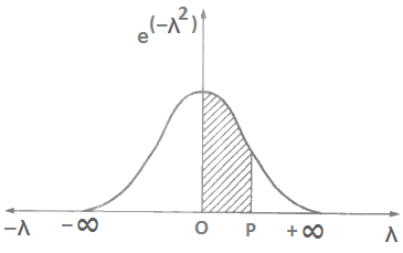
Here λ is an integration variable. It gets deleted when the limits of integral are substituted. The upper limit of the integration is the quantity whose error function is desired. In Eq. (x), p will be the upper limit. The lower limit is always zero.

Curve of error function: Figure 6 shows the plot between e^(–λ2) and λ. The hatched area under the curve from λ = 0 to p gives the value of ‘erf’ in Eq. (x). The area under the curve for λ = 0 to λ, = ± ∞ comes out to be ± √(π/2). Recall Eq. (x) in which 2/π may be called normalization factor.

Standard values of error function: Following values of error function should be kept in mind.

erf(0) = 0,            erf(–∞) = –1

erf(+∞) = +1,       erf(–p) = –erf(p)

Error function of quantity p is given in Table given below.

Applications Based on Second Law

Problems of carburizing, decarburizing, semiconductor doping, corrosion and moisture absorption etc. are solved by second law.

1. Case Hardening (or Carburizing) of Steel: Surfaces of many steel components are hardened by diffusing carbon into them. Objects subjected to dynamic loadings such as gears, wheels of railway engines and coaches, ball and roller bearings etc. have functional requirement of being hard on the outer faces but tough from inside.

They are, therefore, subjected to case hardening or carburizing process in which carbon rich solid, liquid or gas is used. Carbon atoms from solid coke, liquid petroleum or gaseous methane atmosphere diffuse into steel at elevated temperature.

Mechanism of diffusion during carburising: To understand diffusion mechanism during carburization, let the carburizing atmosphere of carbon and steel be at M_c and M_s concentrations respectively, Fig. 7. Initial conditions may be expressed by

M(x,0) = M_s for x>0 ……….(xi)

M(0,t) = M_c               ………..(xii)

On substituting these conditions in Equation (ix), we get

M_s = C₁ – C₂ erf(∞) = C₁ – C₂

and             M_c = C₁ – C₂ erf(0) = C₁ – 0 = C₁

therefore,  M_s = C₁ – C₂ = M_c – C₂

therefore,  C₂ = C₁ – M_s = M_c – M_s ………..(xiii)

If we know M_c, M_s and D_x; then the amount M and depth x of carbon penetration as function of time may be determined from Eq. (ix).

2. Decarburization of Steel: Decarburization is just the opposite of carburization. In this process, the carbon content is reduced from the surface of steel by keeping steel in an oxidizing atmosphere. In doing so, the surrounding oxygen reacts with carbon and produces CO or CO₂ on the surface. The surface layer becomes soft which is responsible for lowering the fatigue resistance of steel.

Therefore, decarburization should be done in non-protective atmosphere such as air. The extent of decarburization and hence amount of decarburized layer to be removed can be determined by using Eq. (ix).

Mechanism of diffusion and its derivation: Refer Fig. 8, in which steel at initial concentration M_s, decarburizes to final concentration M_c. Now consider the following boundary conditions.

M(x,0) = M_s for x<0 ………..(xiv)

M(0,t) = M_c……………………..(xv)

On substituting boundary conditions given by Eq (xiv) in Eq. (ix), we get

M_s = C₁ – C₂ erf(–x/0 ) as x<0

As erf(–∞) = –1, therefore,   M_s = C₁ + C₂

Similarly, boundary conditions given by Eq. (xv) yields

M_c = C₁ – C₂ erf[(0/2) √(D_xt)]

                = C₁ – C₂ erf(0) = C₁

Thus  C₂ = M_s – C₁ = M_s – M_c

Experimental Determination Of Diffusivity

Concept of diffusion couple: Determination of diffusivity is based on the solution of Fick’s second law. Concept of diffusion couple is used for this purpose.

In a diffusion couple, Fig. 9, there are two materials with a common face. The origin O is at interface, and diffusion takes place in direction x. The two materials are at concentrations M₁ and M₂ (M₁ > M₂). The initial conditions for the diffusion couple are:

M(x,0) = M₁(x<0) and M₂(x>0) ……..(xvi)

When sufficient thermal energy is imparted to the diffusion set-up, diffusion starts from material A to material B. Common face depicts concentration at time t = 0. After time t₁ and t₂ the changes in concentration occur about a cross-over point G as shown in Fig. 9. Here the average concentration M bar is

M bar = (M₁ + M₂)/2  …………(xvii)

The concentration-distance profile (M—x profile) is symmetric about G.

Experimental Procedure to Determine Diffusivity: The experiment to determine diffusivity D_x is performed at a predetermined temperature T for a certain time t.

Thin slices perpendicular to the direction x are cut, machined and chemically analyzed to obtain the value of M. In Fig. 9, sections x₁x₁ and x₂x₂ etc. show how to cut the slices.

As x and t are the observed values at known temperature T, initial states M₁, and M₂ are known, hence constants C₁, C₂ and ‘erf’ in Eq. (ix) may be obtained. Thus D_x can be computed.

Diffusivity as a function of temperature: By repeating the experiment at different temperatures, D_x may be obtained as a function of temperature.

D_x = D_oe^(–Q/RT) ………….(viii)

The result given by above equation  is similar to the Arrhenius equation. Here, D_o is a diffusion constant. Values of D_o and Q may be obtained from Arrhenius plot. Values of D_o and Q for some diffusion processes are given in Table.

Diffusion process (Solute in solvent)	Do (10-6 m2/s) At room temperature	Do (10-6 m2/s) At 500oC	Q (kj/mole) At room temperature
Cu in Cu	0.002	1 x 10-18	196
Fe in α-Fe	1.18	1 x 10-20	281
C in α-iron	0.00008	1 x 10-12	83
Cin γ-iron	0.007	5 x 10-15	157
Ni in Fe	0.26	1 x 10-22	295
Cu in Al	0.002	1 x 10-14	120

Factors Affecting Diffusivity

Diffusivity is affected by several factors. Important among them are

Temperature: With an increase in temperature, the diffusivity also increases. This increase is proportional to e^(–1/T) as can be seen from Eq. (xviii). In fact, due to higher temperature, the atoms receive greater thermal energy. Therefore, they can be activated easily to cross-over the energy barrier.

Melting point: Solids having higher melting point possess lower diffusivity. It is because the solids with higher melting point require higher thermal energy to break the bonds.

For example, take the case of Cu-Cu and Cu-Al diffusion. Melting points of Cu and Al are 1083°C and 657°C respectively. It means that Cu-Cu bonds are stronger than Al-Al bonds. That’s why Cu atoms diffuse more easily in Al than in itself.

Atomic packing factor: Highly packed crystals have low diffusivity. We know that APF for FCC and BCC structures are 0.74 and 0.68 respectively. Therefore FCC crystals have lower diffusivity than BCC crystals. That is why diffusion of carbon in BCC-iron is higher than its diffusion in FCC-iron.

Crystal structure: A polycrystalline material shows higher diffusion than a single crystal material at lower temperature. It is due to longer grain boundaries in polycrystalline material which increases diffusion.

However when lattice diffusion dominates at higher temperature, diffusivity becomes the same for polycrystalline and single crystal materials. The distorted crystals show higher diffusivity.

Atomic radius: Materials having smaller atomic radii exhibit higher diffusivity than those having larger atomic radii.

For example, the radii of carbon and nickel atoms are 0.7 ^oA and 1.25 ^oA respectively. Thus carbon atom is much smaller than the nickel atom. Hence diffusivity of carbon in iron is more than that of nickel in iron.

This fact may be noticed in binary solutions where atomic radii of solute and solvent differ significantly. Reason of this situation is the occurrence of interstitial mechanism which requires lower activation energy than the vacancy mechanism.

Grain Size: Fine grained materials have higher diffusivity than coarse gained materials. The reasons may be attributed to grain boundaries. Diffusion through grain boundaries faster and fine grained materials have longer grain boundaries.

Non-crystallanity: Gaseous molecules diffuse faster in non-crystalline structures due to presence of large void space, as in polymers, or due to open network in silicates. Smaller molecules diffuse more rapidly. Use of plasticizer and process of cross-linking have the effects of increasing and decreasing diffusivity respectively.